The first part of this article discussed what databases looked like before Codd’s seminal paper in 1969 introduced the relation model. This post describes what the relational model actually is. By the way, the last article gave some examples from non-relational databases that I’d worked on in the past. I don’t want to give the impression that I was writing software before 1969! Just like there are still plenty of dBase applications still around (what do you mean, “what’s dBase?”) when I was first learning database programming there were still plenty of ISAM applications still running – there probably still are.
Codd’s paper revolutionised the data processing world. Data processing was now based on mathematics. There were now rules which everyone knew and understood. That’s why virtually all databases that you see now are relational and why the old-style ISAM databases disappeared.
So hands up who knows what a relation actually is? Unless you are a computer scientist or mathematician you would probably be wrong. Many people think that relations describe relationships between entities, such as equipment and models. Wrong. A relation is a concept from set theory, which you probably learnt about in junior school.
Suppose we have 2 sets: A = Names and B = Ages. A common way to define the contents of a set is as a comma-separated list between curly brackets. e.g.
A = {Tom, Dick, Harry}
B = {20, 21, 30}
A relation is a new set created by making ordered pairs from all elements of original sets. R1 below is a relation on A and B.
R1 = { {Tom, 20}, {Dick, 21}, {Harry, 30} }
Notice that R1 is itself actually a set which contains:
{
{(the 1st member of set A, the 1st member of set B)},
{(the 2nd member of set A, the 2nd member of set B)}
{(the 3rd member of set A, the 3rd member of set B)}
}
You might see this referred to as:
{
{(A1, B1 )},
{(A2, B2 )},
{(A3, B3 )}
}
The values inside the parentheses are called tuples, or n-tuples and we will see more of them in the next post. In this case n = 2, so these are 2-tuples.
Suppose we had a 3rd set C = Heights:
C = { 5′ 8″, 6′ 2″, 6′ 0″ }
The relation R2 over A, B & C would be:
R2 = { {Tom, 20, 5′ 8″}, {Dick, 21, 6′ 2″}, {Harry, 30, 6′ 0″} }
(In this case the tuples are 3-tuples)
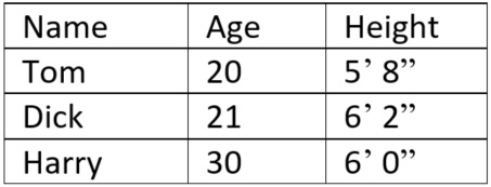
You should now be able to spot how relations are important. Let’s just represent this a different way, with the names of the sets at the top.
We can see now that a relation is effectively a database table. This is the fundamental element that underpins the entire relational database model. RDBMS’s (Relational DataBase Management Systems) all manage data in what have become known as tables, where table is synonymous with relation. All of the data is defined by relations and everything that you can conceivably do to or with these relations is defined by set theory.
Incidentally, RDBMS’s are not the same thing as ROUS’s (Rodents of Unusual Size). They’re a whole different kettle of ballgames, as they say.
Just step back and ponder the enormity of this. We have 3 sets, Names, Ages and Heights, each having the same cardinality (i.e. number of members). By using some fairly elementary maths we can combine those into a mathematical model of the now-familiar concept of a database table. There are some rules that these sets and relations have to follow but the power and flexibility this model gives us is truly amazing (compared with the disadvantages of the older database systems discussed in the last article).
So far this simple relation describes a single, real-world entity, namely a person. Ok, a person is defined by more than their name, age & height, but getting a model that more-closely resembles reality simply involves adding more sets for things like hair colour, shoe size etc. The relational model allows us to define relations for many different entities and to link them together in all kinds of ways.
As an example, let’s look at some set theory and see how this can extend our model. In set theory the Cartesian Product (normally written as “x”) over 2 sets gives a new set containing every element of set 1 combined with every element of set 2.
If:
A = {a, b}
B = {x, y}
Then:
A x B = { {a, x}, {a, y}, {b, x}, {b, y} }
How is this useful? Lets create a new relation, Employers. to list companies that people can work for and rename our earlier relation R2 to People. We can add a new column to the People relation, called Employer.
Employers = { {1, Smiths Ltd}, {2, Browns Ltd} }
People = { {Tom, 1}, {Dick, 1}, {Harry, 2} }
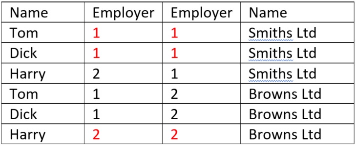
If we take the Cartesian Product of these we get:
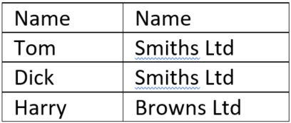
Now we just need to get rid of every row where Employer (from People) doesn’t match Employer (from Employers). This will give (I have got rid of the columns I’m not interested in):
It’s hard to grasp how revolutionary this was back in 1969, now that all databases work like this. We can now keep different lumps of data and combine them using trivial set theory. Each real-world entity (like a person or employer) now only ever needs to be defined once. If Smiths Ltd changes its name to Jones Ltd, that change only needs to be made in a single place, in the employers relation. This is one of the key requirements of properly-designed relational databases: “one fact – one place”.
Set theory contains many operations that let you combine sets (UNION), identify things which several sets have in common (INTERSECTION), subtract one set from another and so on. It would be tiresome for programmers if they had to process data using set-theoretical concepts. Just as high-level programming languages (Fortan, COBOL, C, C++, C#, Pascal, BASIC etc. [Look out- I feel another article coming on!]) shield programmers from having to know how the chips inside the computer work, so high-level data processing languages shield programmers from the grubby maths.
The database world has pretty much decided on a language called SQL (Structured Query Language) to process relational data. There is no consensus as to how this is pronounced; one man’s S-Q-L is another man’s Sequel.
In our simple example above the query “who works where” is expressed in SQL by:
SELECT People.Name, Employers.Name
FROM People INNER JOIN Employers
ON People.Employer = Employers.Employer
If we only wanted to see who works for Smiths Ltd we could add a restriction, such as:
WHERE Employers.Name = Smiths Ltd
This is hiding the mathematical complexities from us and allowing programmers to work in a language which is close to English. However, scratch the surface and the maths is still there.
In the next post I’ll discuss both relational calculus and algebra and dig a bit deeper into what SQL is doing.


